Repository navigation
Tutorials Token Frequency
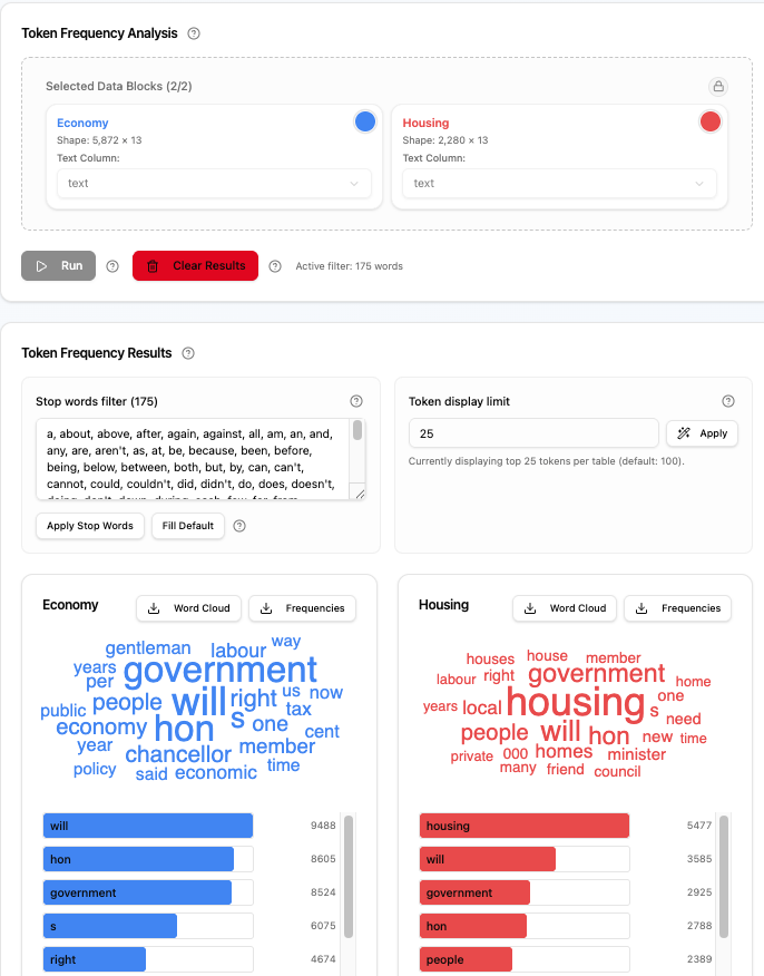
Frequency counts how often each word appears in your text data. It is one of the quickest ways to spot themes and jargon in a corpus. The tool offers two views: Cloud view for a visual impression of the most frequent terms, and List view for a ranked frequency list with precise counts. When two Data Blocks are selected, the tool also produces a comparative keyword analysis (the Juxtorpus cloud) and a statistical measures table that highlight the terms most distinctive to each side.
Use the Data Block selector to choose which corpus (or corpora) to analyse. The tool is strictly pairwise (at most two Data Blocks at a time) because keyword analysis is defined between exactly one Study corpus and one Reference corpus. If more than two Data Blocks are selected in the Project, the tool only shows the two most recent picks; any older selections are silently dropped from the panel until you deselect a newer Data Block to make room.
When two are selected, the tool runs in comparison mode and produces the Juxtorpus cloud and statistical measures in addition to the results for each Data Block.
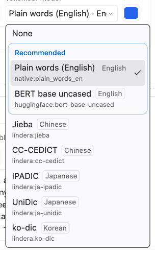
For each selected Data Block, choose the text column that contains the documents you want to count and a tokeniser model that defines the tokens. Only columns that hold plain text are available. Each choice is saved independently on that Data Block and initialises the corresponding control the next time you add it to a fresh Frequency or Concordance selector. If a Data Block has no saved tokeniser preference, Frequency detects the selected column's language and automatically saves the first recommended tokeniser; Jieba is the first recommendation for Chinese text. Plain words splits text at spaces and punctuation and has no trained vocabulary, so it is a baseline for any language that separates words with spaces (English, French, Indonesian, and so on) and the first recommendation for those languages; BERT base uncased is a model trained on English. Clearing one preference does not clear the other. Each tokeniser in the list shows the language it is for, the ones recommended for the detected language are listed first under Recommended, and the link icon beside the selected tokeniser opens its project page in a new tab.
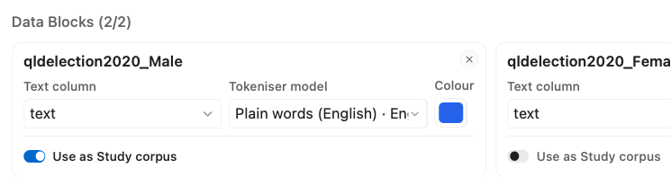
The Colour square on each card sets the colour of that Data Block in the clouds, lists, and Keyword Analysis labels.
Every Frequency run requires a tokeniser model for every selected Data Block. The Analysis stores the exact model mapping it used, so reopening a historical result does not substitute a tokeniser preference that was changed later.
When two Data Blocks are selected, each selected Data Block card shows a Use as Study corpus toggle. Exactly one toggle is on: that Data Block is the Study corpus, and the other Data Block is the Reference corpus. The first Data Block is the Study corpus by default. Turning a toggle on makes its Data Block the Study corpus, and turning the active toggle off makes the other Data Block the Study corpus.
The Study corpus is the collection whose key words you want to find. The Reference corpus is the baseline it is compared against. In the statistics table the Reference corpus appears as OR and %R, and the Study corpus as OS and %S. Directional measures (%DIFF, RRisk, LogRatio, OddsRatio, Overuse, and Signed LL) describe the Study corpus relative to the Reference corpus, so swapping the roles flips their direction.
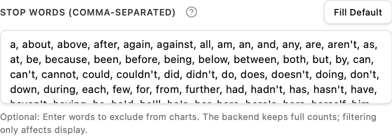
Stop words are terms you want to exclude from the frequency count: commonly words like the, and, or domain-specific filler that would otherwise dominate the results.
- Turn on Enable stop words, then type words separated by commas or newlines. Matching is case-insensitive. Disabling the filter keeps the saved list read-only.
- Pick a list from the dropdown below the switch (Select language, shown as Saved list (N words) once the tab has a list) to append its words to your list (duplicates are skipped, so you can combine lists). The dropdown has three groups: From other tabs (lists saved in your other Frequency and Topic Modelling tabs), Wordflow classic lists (the built-in lists earlier Wordflow versions used, including the revised English list), and Languages (stopword library) (default lists for about 60 languages from the open-source
stopwordpackage). The library group shows only the language detected from the first selected Data Block, marked (Detected); choose Show all languages to see the rest. Choose Clear stop words to start again from an empty list. Picking a list switches the filter on if it was off.
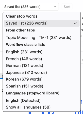
The sources and licences of the ready-made lists are listed under Stop-word lists in the References.
- Lists picked under From other tabs (for example Topic Modelling · 1) are copied into this tab's list; later edits in either tab do not affect the other.
- Click Sort to sort the current stop-word list alphabetically.
- Edits to the list apply when you leave the text box. Removing stop words does not change the statistical measures of remaining tokens: they are excluded as a post-processing step.
- Right-click any word in the word cloud or frequency list to add it directly to the stop-word list. Words added this way are inserted at the start of the list so they are easy to find and remove. The list is not re-sorted until you click Sort.
Choose Run to start. Settings are locked while it works. After it finishes, Run turns on again only when you change a setting that affects the counts. Stop words and the Cloud and List display limits only change what is shown, so they do not turn Run on. See How Preview, Run and Clear work.
The results panel shows controls for stop words and display limits at the top, followed by a shared Filter tokens card and the Cloud view / List view selector. The Enable stop words switch is remembered with the tab, so it stays on across tool switches, reloads, and new runs until you turn it off. Results for each Data Block appear in the same order as the Data Block cards in the parameter panel.
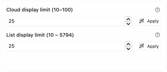
The Cloud display limit (range 10–100, default 50) sets the maximum number of tokens shown in the word clouds. Type a number, or use the arrows, then click Apply. Changing this value also updates the List display limit to the same number (capped at 100).
The List display limit (range 10 to vocabulary size) sets the maximum number of tokens shown in the ranked frequency lists. Values up to 100 stay in sync with the Cloud display limit; setting the list limit above 100 lets you see a longer tail in list view while the cloud remains capped at 100.
The result-level Filter tokens input remains active in both Cloud and List views, with either one or two Data Blocks. Type a pattern to narrow every frequency cloud, frequency list, Juxtorpus cloud, and Keyword Analysis table simultaneously. Filtering searches the full stopword-filtered vocabulary before applying the Cloud or List display limit, so matches outside the original top results remain discoverable. Use * as a wildcard:
-
pre*: all tokens starting with pre -
*ing: all tokens ending in ing -
*ation*: all tokens containing ation
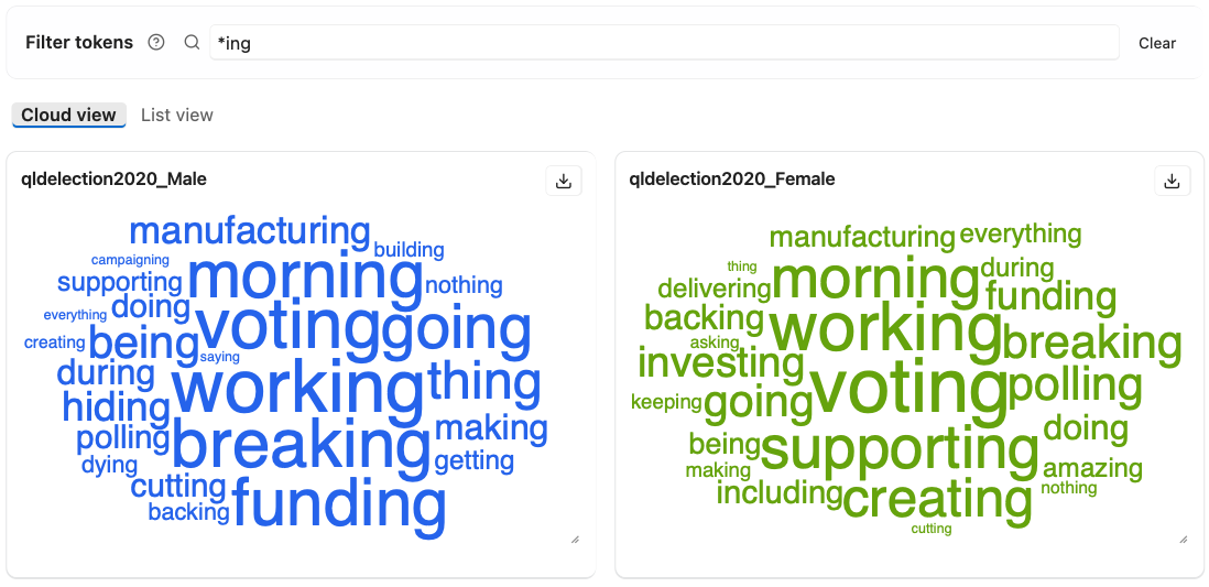
Click Clear to remove the filter. Downloads also follow the active filter: frequency and Keyword Analysis CSVs contain all matching rows, while cloud image exports capture the filtered cloud.
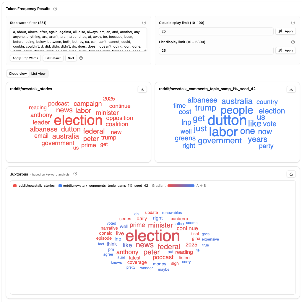
Cloud view shows a word cloud for each selected Data Block, followed by the Juxtorpus cloud when two Data Blocks are selected. The shared token filter applies before the cloud display limit.
Word size in each Data Block's cloud follows frequency, scaled by the square root of each count so that the most frequent words do not crowd out the rest (the counts shown are unchanged). Words are sized to fill the cloud, and they rescale when you resize it. Interaction:
- Left-click any word to jump to the Concordance tab and search for that term in context.
- Right-click any word to add it to the stop-word list (it is inserted at the start of the list).
A download button is available for each cloud (PNG, SVG, or PDF). You can optionally include the associated stop-word list in the download as a zip file.
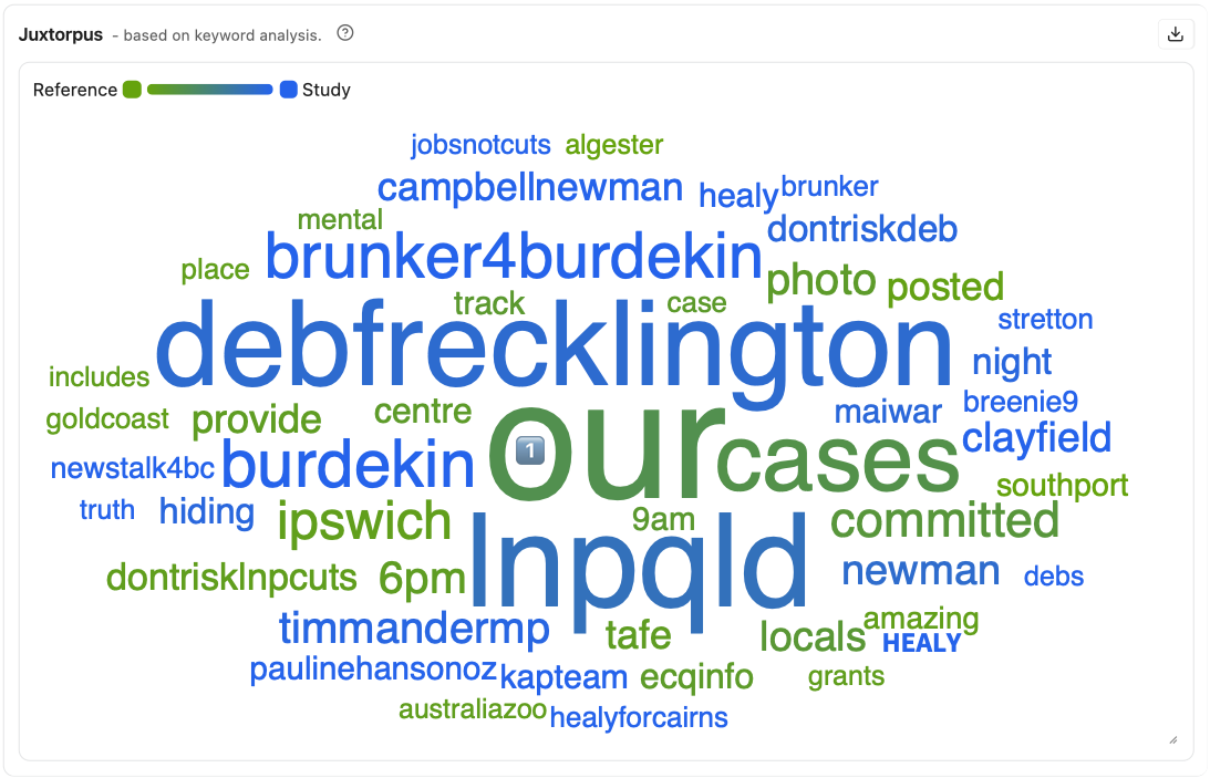
When two Data Blocks are selected, the Juxtorpus cloud appears below the clouds for each Data Block. It highlights the words that are most distinctively used by each Data Block, using the keyword analysis method (log-ratio comparison).
- Size reflects combined frequency across both Data Blocks.
- Colour shifts toward the Data Block where the word has the higher proportional share, so differences in corpus size do not dominate the palette.
- Words are ranked by log₁₀(OS + OR) × LogRatio; the cloud shows the highest and lowest N words by that score (up to twice the cloud display limit).
- The colour bar at the top names the Reference and Study Data Blocks beside their colours. A downloaded Juxtorpus cloud carries the same names and colours in a header and legend, so it can be read outside Wordflow.
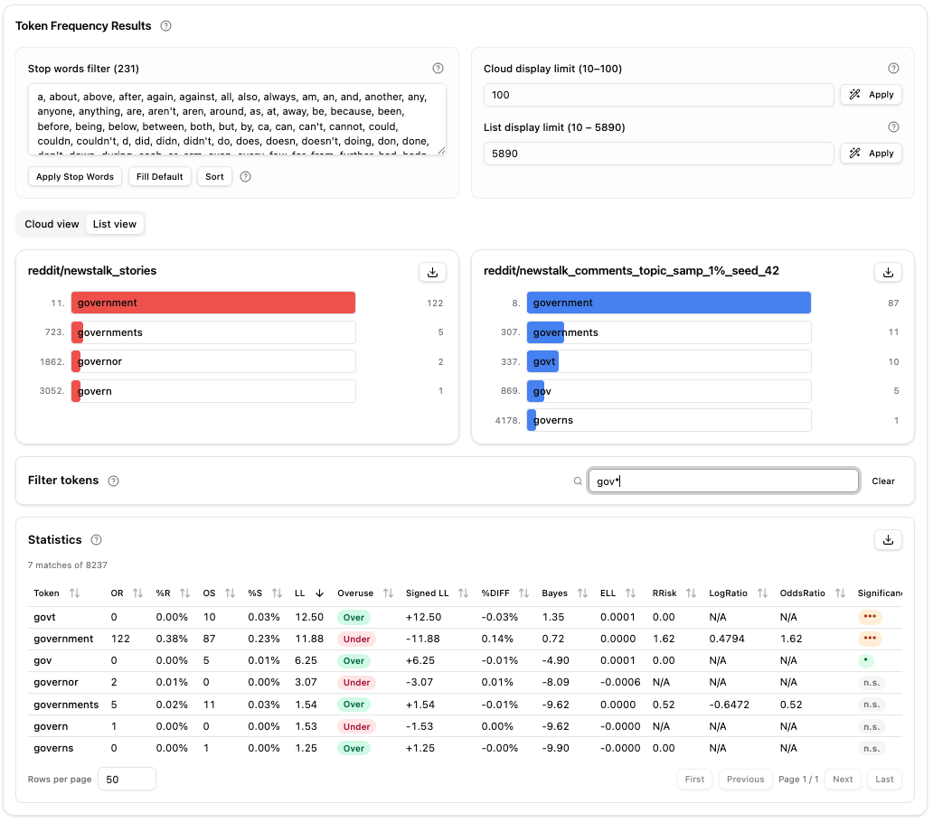
List view shows a ranked horizontal bar chart for each selected Data Block, with the statistics table below when two Data Blocks are compared. The shared token filter applies to the full vocabulary before the list display limit.
Word ranking
Tokens are listed in descending order of frequency. The bar length for each token is proportional to its count relative to the most frequent token in that Data Block. Beside each token, Count is its raw frequency and Per million is its normalised frequency: count ÷ all tokens in the Data Block × 1,000,000, rounded to a whole number. Per million is calculated from every token in the Data Block, so stop words and the token filter do not change it; use it to compare Data Blocks of different sizes. The frequency download includes both columns. When two Data Blocks are shown side by side, the lists are scrolled synchronously: scrolling one list scrolls the other to the same position, making it easy to compare the same rank across both corpora.
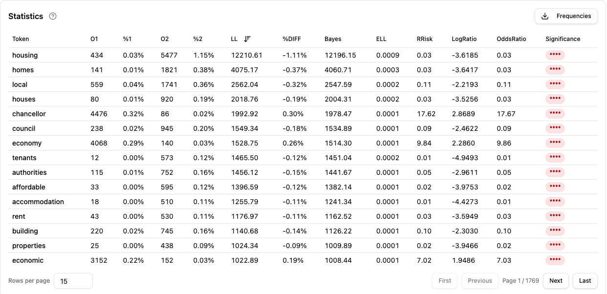
The Keyword Analysis table summarises token-level differences between the Study and Reference corpora. The Reference and Study labels above the table use the chart colour you picked for each Data Block; hover over a label to see the Data Block's name. Hover over any column header for a short explanation, and click it to sort ascending or descending.
| Column | What it shows |
|---|---|
| OR / OS | Observed frequency in the Reference and Study corpora |
| %R / %S | The token's share of all tokens in each Data Block, as a percentage (relative frequency) |
| LL | Log-likelihood (G²): how sure we can be the difference is real. Above 3.84 is significant (p < 0.05) |
| Overuse | Study when the token is relatively more frequent in the Study corpus, otherwise Reference |
| Signed LL | LL, positive for study overuse and negative for study underuse |
| %DIFF | How much more (or less) frequent the token is in the Study corpus, as a percentage |
| Bayes | Bayes factor (BIC): above 2 is positive evidence, above 6 strong, above 10 very strong |
| ELL | Effect size for log-likelihood |
| RRisk | Relative risk: study relative frequency divided by reference relative frequency |
| LogRatio | Binary log of RRisk: 1 means twice as frequent in the Study corpus, −1 half as frequent |
| OddsRatio | Odds of the token in the Study corpus divided by its odds in the Reference corpus |
| Significance | **** p < 0.0001, *** p < 0.001, ** p < 0.01, * p < 0.05, n.s. not significant (shown below the table too) |
For a token, OS and OR are its counts in the Study and Reference corpora, NS and NR are the corpora's total token counts, and N = NS + NR.
- Relative frequency: %S = OS ÷ NS × 100 and %R = OR ÷ NR × 100.
- Expected frequencies: ES = NS × (OS + OR) ÷ N, and ER likewise with NR.
- LL = 2 × (OS × ln(OS ÷ ES) + OR × ln(OR ÷ ER)), where a zero count adds nothing (Rayson and Garside 2000). The significance stars use the critical values 3.84, 6.63, 10.83, and 15.13.
- %DIFF = (%S − %R) ÷ %R × 100 (Gabrielatos and Marchi 2012). A token that never occurs in the Reference corpus has no %DIFF (shown as N/A).
- Bayes (BIC) = LL − ln(N) (Wilson 2013).
- ELL = LL ÷ (N × ln(the smaller of ES and ER)) (Johnston et al. 2006).
- RRisk = %S ÷ %R.
- LogRatio = log₂(%S ÷ %R), counting a zero frequency as 0.5 so the ratio stays finite (Hardie 2014).
- OddsRatio = (OS ÷ (NS − OS)) ÷ (OR ÷ (NR − OR)).
Results created before Wordflow 0.7.8 measured the Reference corpus against the Study corpus, so their %DIFF, RRisk, LogRatio, and OddsRatio are reversed. Run the analysis again to get the current direction.
The table is paged: use Words per page and the page controls below it. Sorting always applies to the whole table before paging, and N/A values stay at the bottom whichever way you sort.
The full table can be downloaded as a CSV file, in the order the table is sorted; when the shared token filter is active, the download contains all matching rows. The CSV uses the same column names as the table, with each corpus's name added (for example OR_speeches), plus Expected_…, the count the token would have in that corpus if both corpora used it equally, and Total_…, the corpus's total number of tokens. For further reading on keyword analysis methodology, see the Lancaster corpus linguistics resource and Paul Rayson's log-likelihood and effect size calculator, which these formulas follow.
The tab keeps its result when you move to another tool or reopen the Project. Clear removes it and resets the tab. After a failure or a stop, the settings stay editable but Run stays off until you choose Clear. See How Preview, Run and Clear work.
| Symptom | Likely cause | What to try |
|---|---|---|
| Results unchanged after removing stop words | Filter off, or the text box still has focus | Turn on the stop words switch, then click outside the text box to apply your edits |
| Word cloud dominated by common words | No stop words applied | Pick your corpus language from the stop words Select language dropdown |
| Juxtorpus or Keyword Analysis table are missing | Only one Data Block selected | Select a second Data Block to enable comparison mode |
| Keyword Analysis table shows no significant words | Corpora are very similar or one is very small | Try a larger or more distinct pair of Data Blocks |
| A Data Block I selected isn't showing in the panel | Frequency caps the panel to the 2 most-recent selections | Deselect a newer Data Block to make room, or run the comparison on the visible pair |
| Right-clicked stop word is hard to find | List was already long when the word was added | New words are inserted at the top: scroll to the start, or click Sort to alphabetise |
| Run button is disabled | No Data Block, text column, or tokeniser model selected | Select a Data Block, text column, and tokeniser model |
| Setting | Default | Notes |
|---|---|---|
| Data Blocks | None | Up to 2; comparison mode activates when 2 are selected. If more than 2 are selected Project-wide, only the 2 most recent show in the panel. |
| Tokeniser model | Saved Data Block preference or none | Required for each selected Data Block; the submitted Analysis freezes the exact mapping |
| Corpus role switches | First selected Data Block is the Study corpus | Swaps which Data Block is OS/%S and which is OR/%R in the statistics table |
| Stop words | Empty | Pick a language from the Select language dropdown for default stop words |
| Token filter | Empty | Applies to every Cloud/List result and download; * matches any sequence of characters |
| Cloud display limit | 50 | Range 10–100; mirrors to list limit |
| List display limit | 50 | Range 10 to vocabulary size; values > 100 diverge from cloud |
- Select a Data Block and click Run with the default settings.
- Pick the detected language from the stop words Select language dropdown to add its default stop words, and compare the top tokens.
- Right-click one of the remaining high-frequency words in the cloud to add it as a custom stop word. The stop words filter switches on automatically if it was off. Confirm the word appears at the start of the stop-word list.
- Select a second Data Block. Use the card-level Use as Study corpus toggles to choose the Study corpus (the other Data Block becomes the Reference corpus), then choose Run again.
- Use Filter tokens with a wildcard pattern (e.g.
*ing) and confirm that Cloud view, List view, and their downloads remain filtered while switching views. - In List view, scroll one frequency list and observe that the other list scrolls in sync.
- Sort the statistics table by LogRatio to find the words most distinctively associated with each Data Block.
- Left-click one of the top distinctive words to jump to Concordance and inspect it in context.